Physically Based Rendering Algorithms: A Comprehensive Study In Unity3D - Part 2 - Piecing Together Your PBR Shader

The Normal Distribution Function (Specular Function)

What is the Normal Distribution Function?

The Normal Distribution Function is one of the three key elements that make up our BRDF shader. The NDF statistically describes the distribution of microfacet normals on a surface. For our uses, the NDF serves as a weighted function to scale the brightness of reflections (specularity). It is important to think of the NDF as a fundemental geometric property of the surface. Let's start to add some algorithms to our shader, so that we can visualize the effect that the NDF produces.

The first thing we want to do is build an algorithm. In order to visualize our algorithm, we will override our return float.

float3 SpecularDistribution = specColor;

//the algorithm implementations will go here

return float4(float3(1,1,1) * SpecularDistribution.rgb,1);

The format for the following sections will be as follows. After your write the algorithm in the Algorithm Section, you will implement the algorithm in the location described above. When you implement a new algorithm, simply comment out the above active algorithm, and the resulting effect will be based on only the currently uncommented algorithm. Don't worry, we will clean this up later and provide you with a way to easily switch between the algorithms from within Unity, no further comment play required.

Let's start with the simple Blinn-Phong approach:

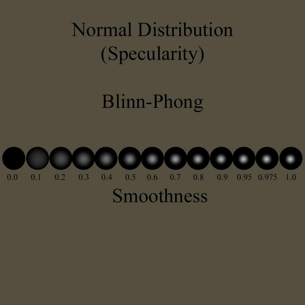
Blinn-Phong NDF

The Blinn approximation of Phong specularity was created as an optimization of the Phong Specular Model. Blinn decided that it was faster to produce the dot product of the normal and half vector, than it was to calculate the reflect vector of light every frame. The algorithms do produce much different results, with Blinn being softer than Phong.

float BlinnPhongNormalDistribution(float NdotH, float specularpower, float speculargloss){
    float Distribution = pow(NdotH,speculargloss) * specularpower;
    Distribution *= (2+specularpower) / (2*3.1415926535);
    return Distribution;
}

Blinn-Phong is not considered a physically correct algorithm, but it will still produce reliable specular highlights that can be used for specific artistic intentions. Place the above algorithm in the Algorithms Section, and the below code in the Fragment Section.

SpecularDistribution *=  BlinnPhongNormalDistribution(NdotH, _Glossiness,  max(1,_Glossiness * 40));

If you assign a smoothness value to your shader, you should see that the object will have a white highlight depicting the Normal Distribution (Specularity) and the rest of the object will be black. This is how we will continue to function, so that we can easily test our shader. The 40 in the above implementation is just so that I could provide the function with a high range, but it most certainly isn't the optimal value for everyone.

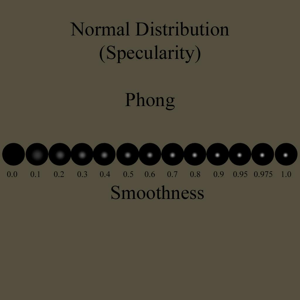
Phong NDF

float PhongNormalDistribution(float RdotV, float specularpower, float speculargloss){
    float Distribution = pow(RdotV,speculargloss) * specularpower;
    Distribution *= (2+specularpower) / (2*3.1415926535);
    return Distribution;
}

The Phong algorithm is another non-physical algorithm, but it produces much finer results than the above Blinn approximation. Below is an example implementation:

SpecularDistribution *=  PhongNormalDistribution(RdotV, _Glossiness, max(1,_Glossiness * 40));

As with the Blinn-Phong approach, don't be sold on the *40.

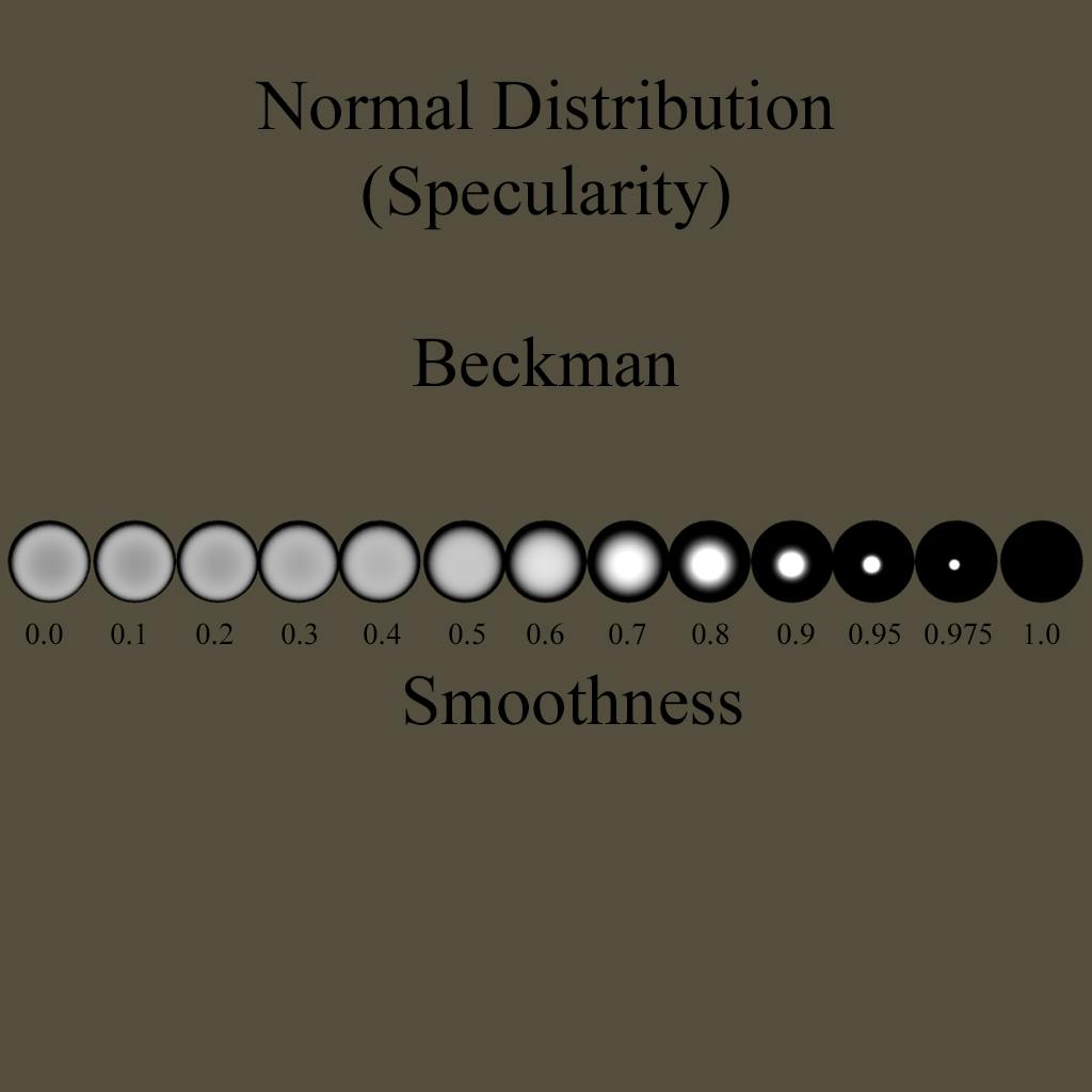
Beckman NDF

The Beckman Normal Distribution function is a much more advanced function, and takes our roughness value into account. Accounting for the roughness, as well as the dot product between our normal and half direction, we can accurately approximate the distribution of the normal across the surface.

float BeckmannNormalDistribution(float roughness, float NdotH)
{
    float roughnessSqr = roughness*roughness;
    float NdotHSqr = NdotH*NdotH;
    return max(0.000001,(1.0 / (3.1415926535*roughnessSqr*NdotHSqr*NdotHSqr))
* exp((NdotHSqr-1)/(roughnessSqr*NdotHSqr)));
}

The implementation of this Algorithm is failry simple.

SpecularDistribution *=  BeckmannNormalDistribution(roughness, NdotH);

An important thing to note is how the Beckman model treats the surface of the object. As you can tell in the figure above, the Beckman model is slow to change with the smoothness value, until a certain point at which it tightens the highlight dramatically. As the smoothness of the surface increases, the specular highlight pulls together, producing a very pleasing rough to smooth value from an artistic perspective. This behavior is very favorable for rough metals in the early roughness values, and also quite good for plastics as the smoothness value increases.

Gaussian NDF

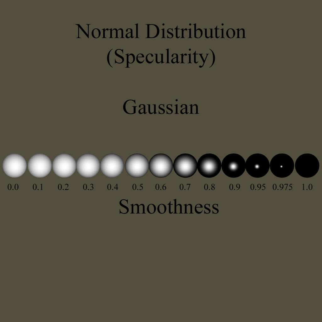
The Gaussian Normal Distribution model is not as popular as some of the other models, as it tends to produce much softer specular highlights than can be desired at higher smoothness values. From an artistic perspective this can be desirable, but there are arguments as to its true physical nature.

float GaussianNormalDistribution(float roughness, float NdotH)
{
    float roughnessSqr = roughness*roughness;
	float thetaH = acos(NdotH);
    return exp(-thetaH*thetaH/roughnessSqr);
}

The implementation of this algorithm is similar to that of other Normal Distribution functions, relying on the roughness of the surface and the dot product of the Normal and Half Vectors.

SpecularDistribution *=  GaussianNormalDistribution(roughness, NdotH);

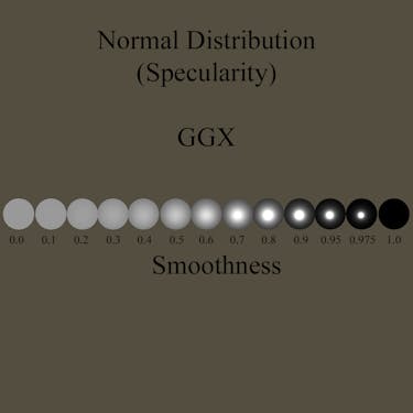
GGX NDF

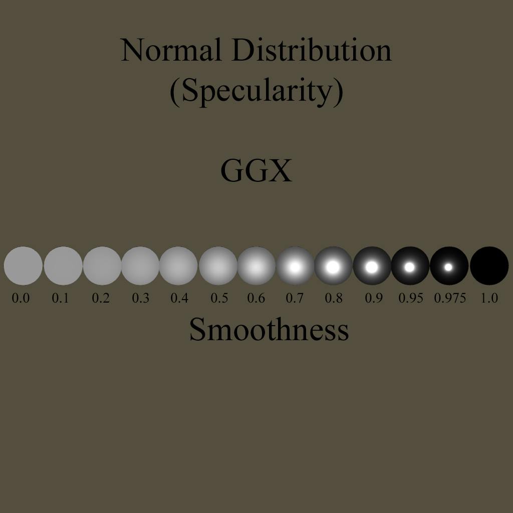
GGX is one of the more popular, if not the most popular, algorithms in use today. The majority of modern applications rely on it for several of their BRDF functions. GGX was developed by Bruce Walter and Kenneth Torrance. Many of the algorithms in their paper are some of the more popular algorithms in use.

float GGXNormalDistribution(float roughness, float NdotH)
{
    float roughnessSqr = roughness*roughness;
    float NdotHSqr = NdotH*NdotH;
    float TanNdotHSqr = (1-NdotHSqr)/NdotHSqr;
    return (1.0/3.1415926535) * sqr(roughness/(NdotHSqr * (roughnessSqr + TanNdotHSqr)));
}

It's implementation follows suit to other methods.

SpecularDistribution *=  GGXNormalDistribution(roughness, NdotH);

The specular highlight of the GGX Algorithm is very tight and hot, while still maintaining a smooth distribution across the surface of our ball. This is a prime example of why the GGX algorithm is preferred to replicate the distortion of specularity across metallic surfaces.

Trowbridge-Reitz NDF

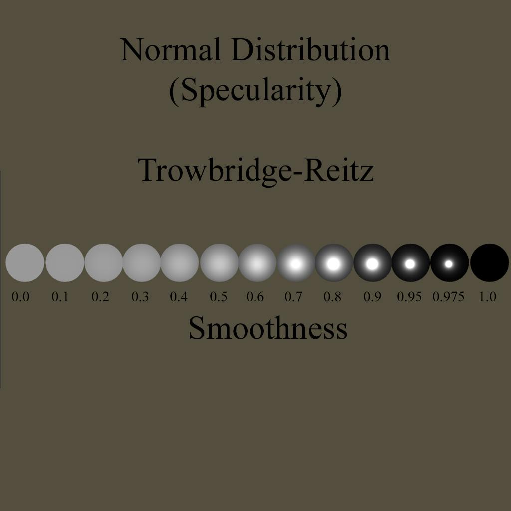
The Trowbridge-Reitz approach was developed in the same paper as GGX, and produces remarkably similar results to the GGX algorithm. The main noticeable difference is that the extreme edge of the object features a smoother highlight than the GGX, which is a more harsh falloff at the grazing angle.

float TrowbridgeReitzNormalDistribution(float NdotH, float roughness){
    float roughnessSqr = roughness*roughness;
    float Distribution = NdotH*NdotH * (roughnessSqr-1.0) + 1.0;
    return roughnessSqr / (3.1415926535 * Distribution*Distribution);
}

As usual, the Trowbridge-Reitz formula relies on roughness and the dot product of the normal and half vectors.

SpecularDistribution *=  TrowbridgeReitzNormalDistribution(NdotH, roughness);

Trowbridge-Reitz Anisotropic NDF

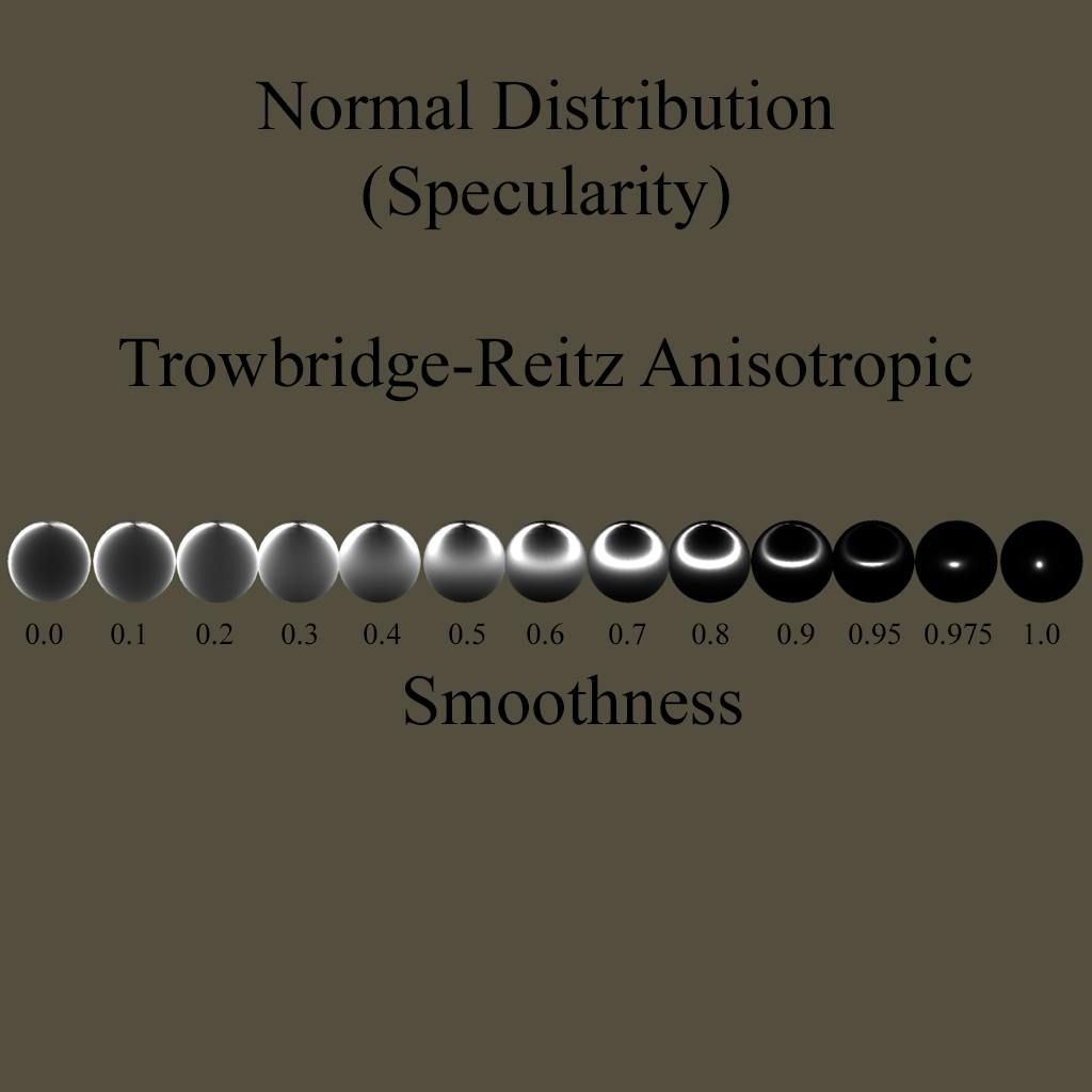
Anisotropic NDF functions produce the normal distribution Anisotropically. This allows for us to create surface effects that mimic brushed metals and other finely faceted/anisotropic surfaces. For this function we will need to add a variable to our Properties and Public Variables Sections.

Our Property:

_Anisotropic("Anisotropic",  Range(-20,1)) = 0

Our Variable:

float _Anisotropic;

float TrowbridgeReitzAnisotropicNormalDistribution(float anisotropic, float NdotH, float HdotX, float HdotY){

    float aspect = sqrt(1.0h-anisotropic * 0.9h);
    float X = max(.001, sqr(1.0-_Glossiness)/aspect) * 5;
    float Y = max(.001, sqr(1.0-_Glossiness)*aspect) * 5;
    
    return 1.0 / (3.1415926535 * X*Y * sqr(sqr(HdotX/X) + sqr(HdotY/Y) + NdotH*NdotH));
}

One of the differences between Anisotropic and Isotropic approaches is the necessity of tangent and binormal data to process the direction of the normal distribution. This image was produced with an Anisotropic value of 1.

SpecularDistribution *=  TrowbridgeReitzAnisotropicNormalDistribution(_Anisotropic,NdotH, 
dot(halfDirection, i.tangentDir), 
dot(halfDirection,  i.bitangentDir));

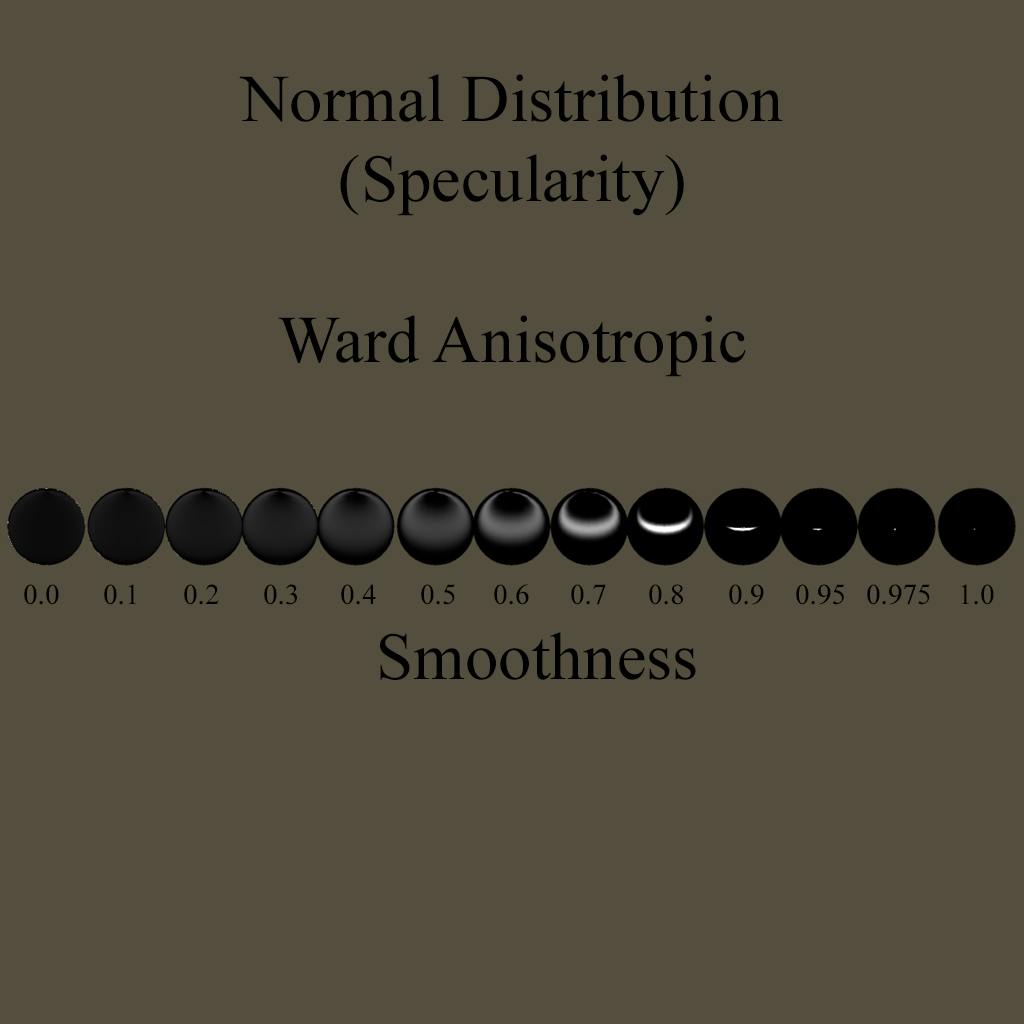
Ward Anisotropic NDF

The Ward approach to Anisotropic BRDF produces drastically different results than the Trowbridge-Reitz method. The Specular highlight is much softer, and dissapates much faster as the surface proceeds in smoothness.

float WardAnisotropicNormalDistribution(float anisotropic, float NdotL,
 float NdotV, float NdotH, float HdotX, float HdotY){
    float aspect = sqrt(1.0h-anisotropic * 0.9h);
    float X = max(.001, sqr(1.0-_Glossiness)/aspect) * 5;
 	float Y = max(.001, sqr(1.0-_Glossiness)*aspect) * 5;
    float exponent = -(sqr(HdotX/X) + sqr(HdotY/Y)) / sqr(NdotH);
    float Distribution = 1.0 / (4.0 * 3.14159265 * X * Y * sqrt(NdotL * NdotV));
    Distribution *= exp(exponent);
    return Distribution;
}

As with the Trowbridge-Reitz method, the Ward Algorithm requires tangent and bitangent data, but also relies on the dot product of the normal and light, as well as the dot product of the normal and our viewpoint.

SpecularDistribution *=  WardAnisotropicNormalDistribution(_Anisotropic,NdotL, NdotV, NdotH, 
dot(halfDirection, i.tangentDir), 
dot(halfDirection,  i.bitangentDir));

We've covered the primary algorithms that represent Normal Distribution Functions. In the next article we will go through the different Geometric Shadowing Functions, which define how microfacets self shadow and affect the attenuation of light on a surface.