Physically Based Rendering Algorithms: A Comprehensive Study In Unity3D - Part 3 - Piecing Together Your PBR Shader

Piecing Together Your PBR Shader Pt.2: The Geometric Shadowing Function

What are Geometric Shadowing Algorithms?

The Geometric Shadowing Function is used to describe the attenuation of the light due to the self-shadowing behavior of microfacets. This approximation models the probability that at a given point the microfacets are occluded by each other, or that light bounces on multiple microfacets. During these probabilities, light loses energy before reaching the viewpoint. In order to accurately generate a GSF, one must sample roughness to determine the microfacet distribution. There are several functions that do not include roughness, and while they still produce reliable results, they do not fit as many use cases as the functions that do sample roughness.

The Geometric Shadowing Function is essential for BRDF energy conservation. Without the GSF, the BRDF can reflect more light energy than it receives. A key part of the microfacet BRDF equation relates to the ratio between the active surface area (the area covered by surface regions that reflect light energy from L to V) and the total surface area of the microfaceted surface. If shadowing and masking are not accounted for, then the active area may exceed the total area, which can lead to the BRDF not conserving energy, in some cases by drastic amounts.

 float GeometricShadow = 1;

//the algorithm implementations will go here

 return float4(float3(1,1,1) * GeometricShadow,1);

In order to preview our GSF functions, let's place this code above our Normal Distribution Functions. The format will work in a very similar way to how we implemented the NDF functions.

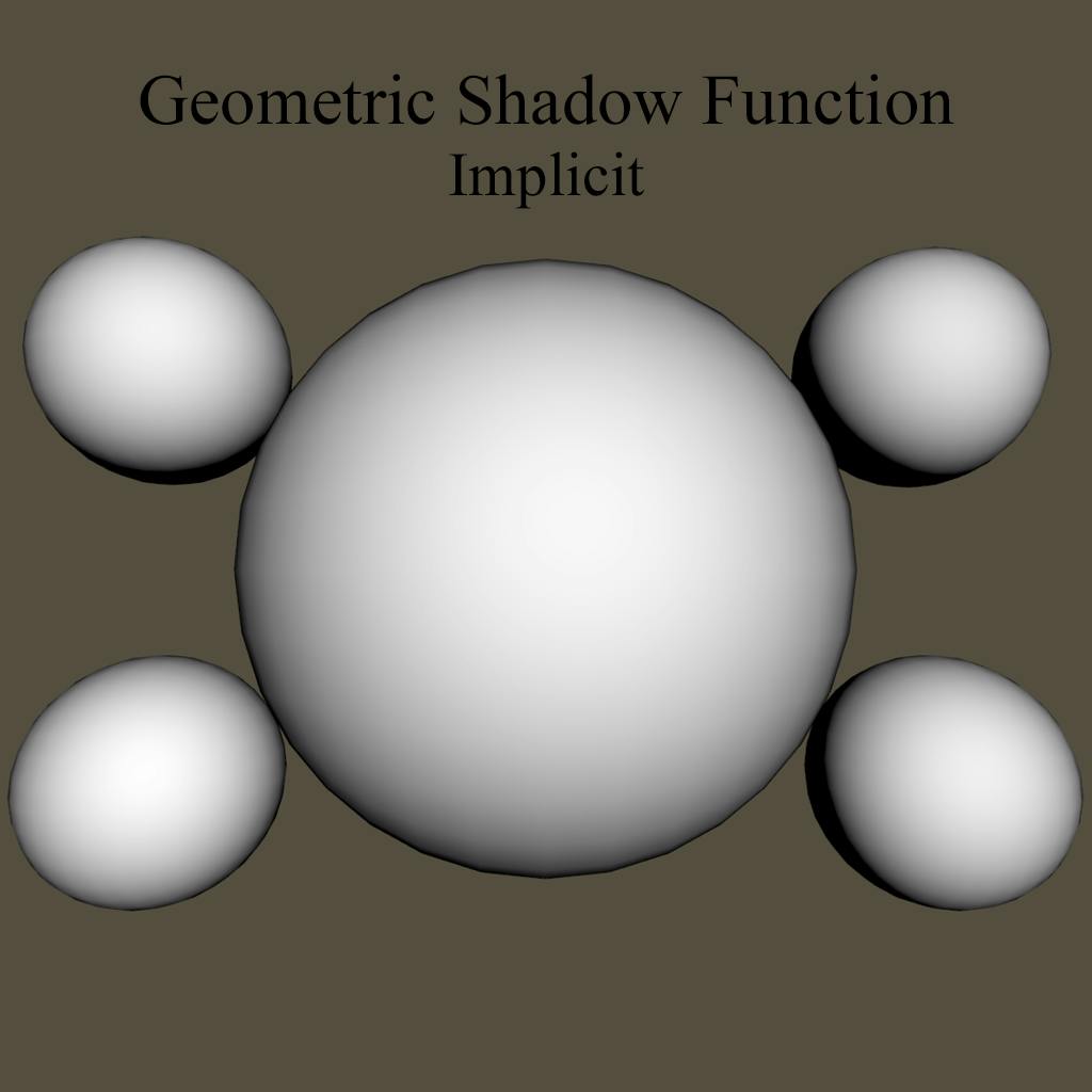
Implicit GSF

The Implicit GSF is the basis of logic behind Geometric Shadowing.

float ImplicitGeometricShadowingFunction (float NdotL, float NdotV){
	float Gs =  (NdotL*NdotV);       
	return Gs;
}

By multiplying the dot product of the normal and light by the dot product of the normal and our viewpoint we get an accurate portrayal of how light affects the surface of an object based on our view.

GeometricShadow *= ImplicitGeometricShadowingFunction (NdotL, NdotV);

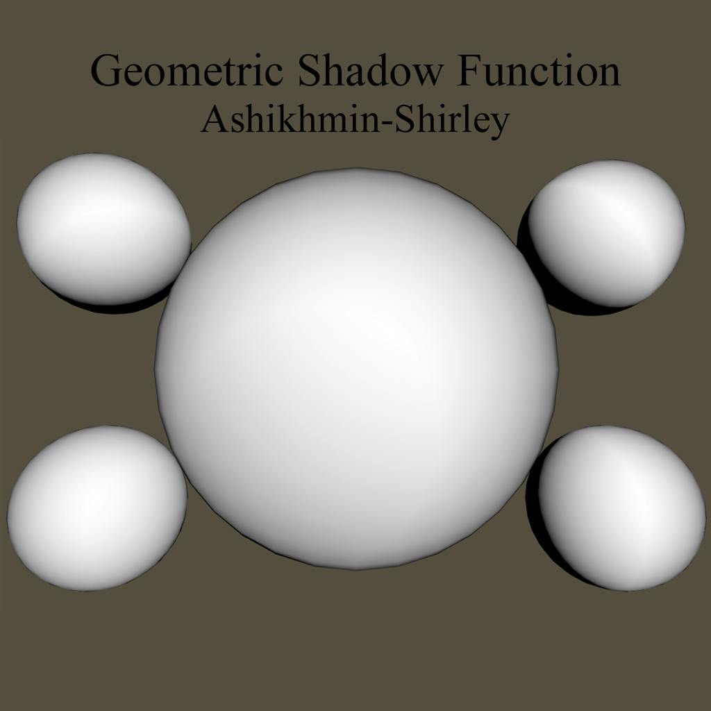
Ashikhmin-Shirley GSF

Designed for use with Anisotropic Normal Distribution Functions, the Ashikhmin-Shirley GSF provides a good foundation for Anisotropic effects.

float AshikhminShirleyGSF (float NdotL, float NdotV, float LdotH){
	float Gs = NdotL*NdotV/(LdotH*max(NdotL,NdotV));
	return  (Gs);
}

The shadowing of microfacets produced by this model is very subtle, as can be seen on the right.

GeometricShadow *= AshikhminShirleyGSF (NdotL, NdotV, LdotH);

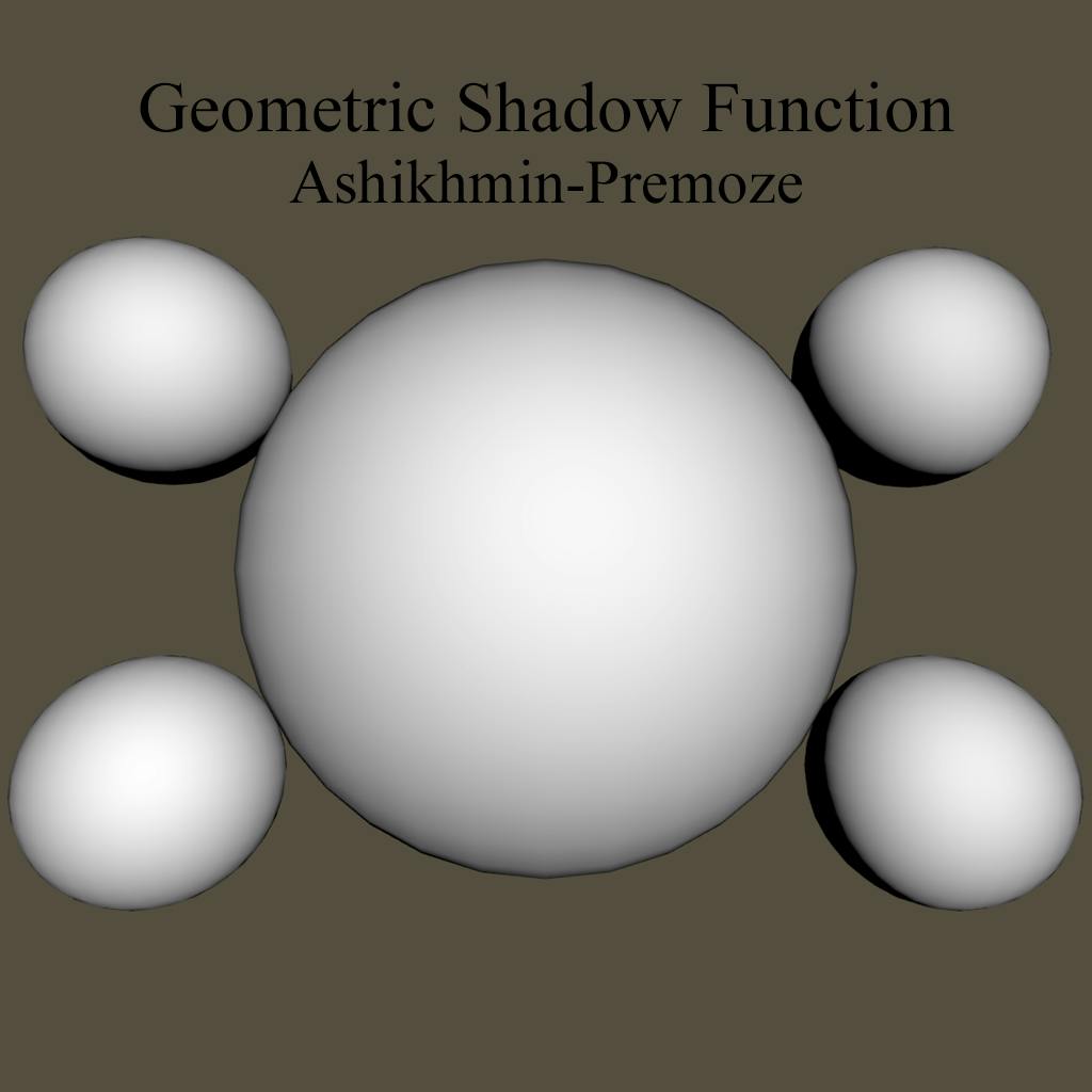
Ashikhmin-Premoze GSF

The Ashikhmin-Premoze GSF is designed for use with Isotropic NDF, unlike the Ashikhmin-Shirley approach. As with the Ashikhmin-Shirley, this is a very subtle GSF.

float AshikhminPremozeGeometricShadowingFunction (float NdotL, float NdotV){
	float Gs = NdotL*NdotV/(NdotL+NdotV - NdotL*NdotV);
	return  (Gs);
}

GeometricShadow *= AshikhminPremozeGeometricShadowingFunction (NdotL, NdotV);

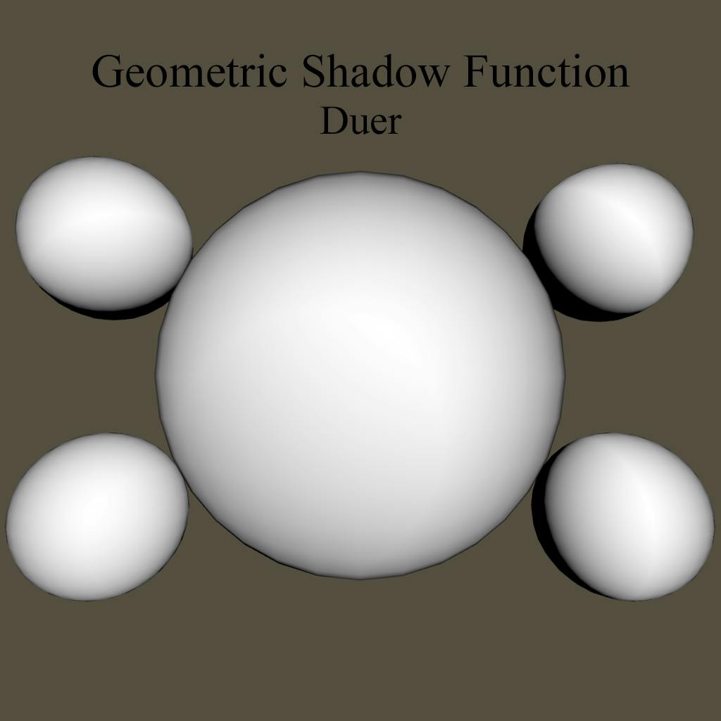
Duer GSF

Duer proposed the GSF function below to fix an issue with specularity found in the Ward GSF function we will cover later. The Duer GSF produces similar results as the Ashikhmin-Shirley above, but is more suited towards Isotropic BRDFs, or very slightly Anisotropic BRDF.

float DuerGeometricShadowingFunction (float3 lightDirection,float3 viewDirection, 
float3 normalDirection,float NdotL, float NdotV){
    float3 LpV = lightDirection + viewDirection;
    float Gs = dot(LpV,LpV) * pow(dot(LpV,normalDirection),-4);
    return  (Gs);
}

GeometricShadow *= DuerGeometricShadowingFunction (lightDirection, viewDirection, normalDirection, NdotL, NdotV);

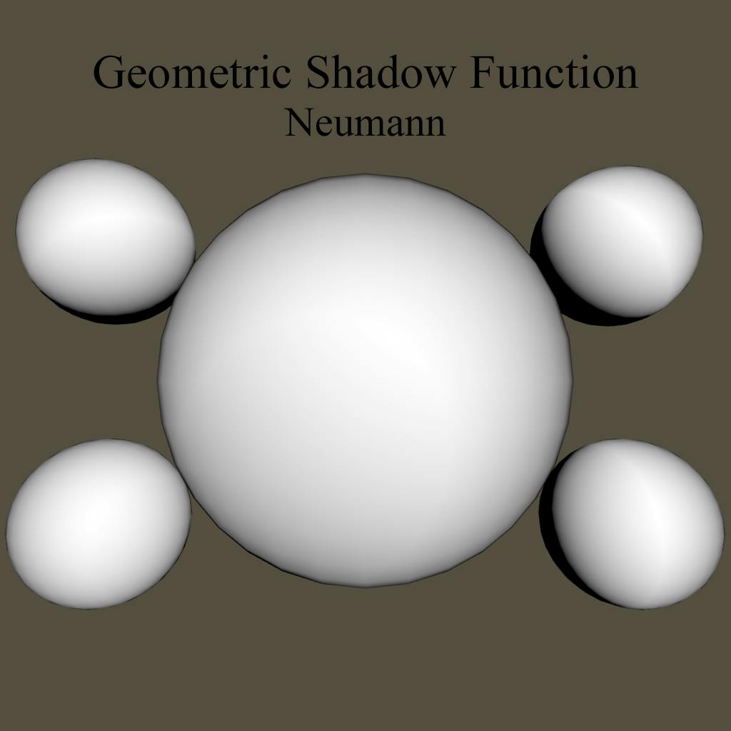
Neumann GSF

The Neumann-Neumann GSF is another example of a GSF suited for Anisotropic Normal Distribution. It produces more pronounced geometric shading based on the greater of view direction or light direction.

float NeumannGeometricShadowingFunction (float NdotL, float NdotV){
	float Gs = (NdotL*NdotV)/max(NdotL, NdotV);       
	return  (Gs);
}

GeometricShadow *= NeumannGeometricShadowingFunction (NdotL, NdotV);

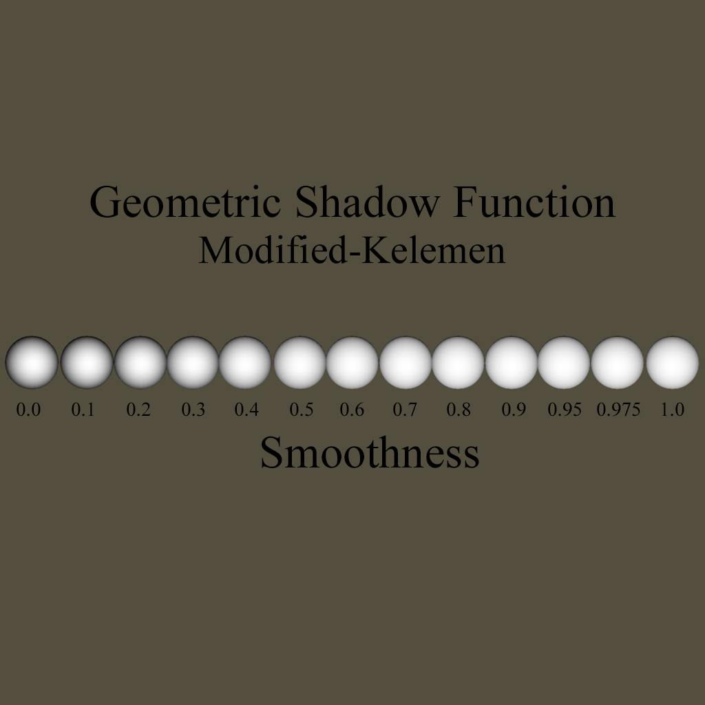
Kelemen GSF

The Kelemen GSF presents an appropriately energy conserving GSF. Unlike most of the previous models, the proportion of the Geometric Shadow is not constant but varies with the viewing angle. This is an extreme Approximation of the Cook-Torrance Geometric Shadowing Function.

float ModifiedKelemenGeometricShadowingFunction (float NdotV, float NdotL,
 float roughness)
{
	float c = 0.797884560802865;    // c = sqrt(2 / Pi)
	float k = roughness * roughness * c;
	float gH = NdotV  * k +(1-k);
	return (gH * gH * NdotL);
}

GeometricShadow *=  ModifiedKelemenGeometricShadowingFunction (NdotV, NdotL, roughness );

Cook-Torrance GSF

The Cook-Torrance GSF was created to solve three situations of Geometric attenuation. The first case states that the light is reflected without interference,while the second case states that some of the reflected light is blocked after reflection, and the third case states that some of the light is blocked before reaching the next microfacet. To compute these cases we use the Cook-Torrance GSF below.

float CookTorrenceGeometricShadowingFunction (float NdotL, float NdotV, 
float VdotH, float NdotH){
	float Gs = min(1.0, min(2*NdotH*NdotV / VdotH, 
2*NdotH*NdotL / VdotH));
	return  (Gs);
}

GeometricShadow *= CookTorrenceGeometricShadowingFunction (NdotL, NdotV, VdotH, NdotH);

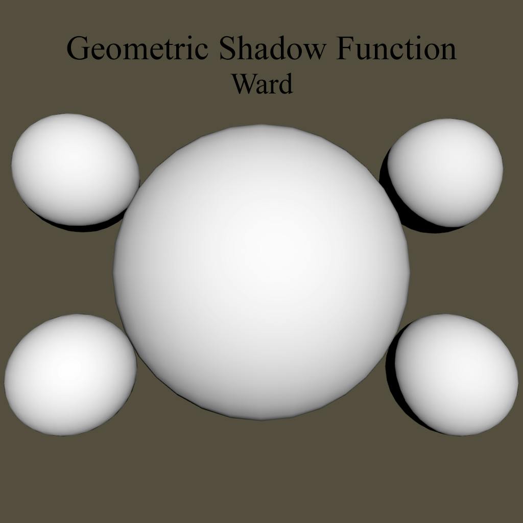
Ward GSF

The Ward GSF is a strengthened Implicit GSF. Ward uses this approach to strengthen the Normal Distribution Function. It works particularly well to highlight Anisotropic bands on surfaces from varying angles of view.

float WardGeometricShadowingFunction (float NdotL, float NdotV, 
float VdotH, float NdotH){
	float Gs = pow( NdotL * NdotV, 0.5);
	return  (Gs);
}

GeometricShadow *= WardGeometricShadowingFunction (NdotL, NdotV, VdotH, NdotH);

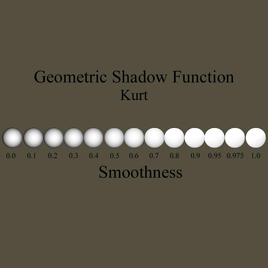
Kurt GSF

The Kurt GSF is another example of an Anisotropic GSF. This model is proposed to help control the Distribution of Anisotropic surfaces based on the surface roughness. This model seeks to conserve energy particularly along the grazing angles.

float KurtGeometricShadowingFunction (float NdotL, float NdotV, 
float VdotH, float roughness){
	float Gs =  NdotL*NdotV/(VdotH*pow(NdotL*NdotV, roughness));
	return  (Gs);
}

GeometricShadow *= KurtGeometricShadowingFunction (NdotL, NdotV, VdotH, roughness);

Smith Based Geometric Shadowing Functions

The Smith Based GSFs are widely considered to be more accurate than the other GSFs, and take into account the roughness and shape of the normal distribution. These functions require two pieces to be processed in order to compute for the GSF.

Walter et all. GSF

The common form of the GGX GSF, Walter et al. created this function to be used with any NDF. Walter et al. felt that the GSF "has relatively little effect on the shape of the BSDF [Bi-Directional Scattering Distribution Function], except near grazing angles or for very rough surfaces, but is needed to maintain energy conservation." With this in mind, they created a GSF that respected this principle, using Roughness as a driving force for the GSF.

float WalterEtAlGeometricShadowingFunction (float NdotL, float NdotV, float alpha){
    float alphaSqr = alpha*alpha;
    float NdotLSqr = NdotL*NdotL;
    float NdotVSqr = NdotV*NdotV;

    float SmithL = 2/(1 + sqrt(1 + alphaSqr * (1-NdotLSqr)/(NdotLSqr)));
    float SmithV = 2/(1 + sqrt(1 + alphaSqr * (1-NdotVSqr)/(NdotVSqr)));


	float Gs =  (SmithL * SmithV);
	return Gs;
}

GeometricShadow *= WalterEtAlGeometricShadowingFunction (NdotL, NdotV, roughness);

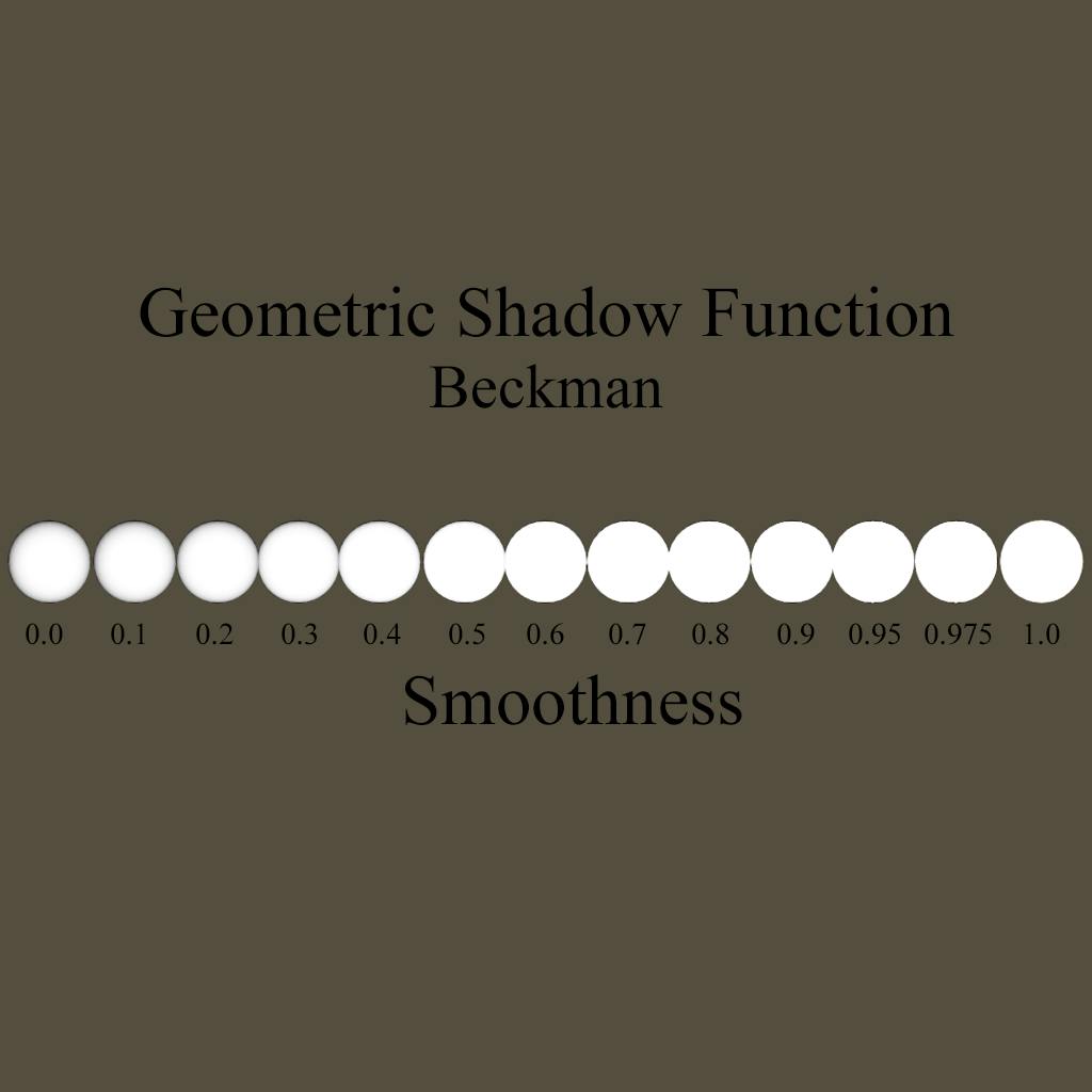
Smith-Beckman GSF

Originally created to be used with the Beckman NDF, Walter et al. surmised that it is an appropriate GSF for use with the Phong NDF.

float BeckmanGeometricShadowingFunction (float NdotL, float NdotV, float roughness){
    float roughnessSqr = roughness*roughness;
    float NdotLSqr = NdotL*NdotL;
    float NdotVSqr = NdotV*NdotV;


    float calulationL = (NdotL)/(roughnessSqr * sqrt(1- NdotLSqr));
    float calulationV = (NdotV)/(roughnessSqr * sqrt(1- NdotVSqr));


    float SmithL = calulationL < 1.6 ? (((3.535 * calulationL)
 + (2.181 * calulationL * calulationL))/(1 + (2.276 * calulationL) + 
(2.577 * calulationL * calulationL))) : 1.0;
    float SmithV = calulationV < 1.6 ? (((3.535 * calulationV) 
+ (2.181 * calulationV * calulationV))/(1 + (2.276 * calulationV) +
 (2.577 * calulationV * calulationV))) : 1.0;


	float Gs =  (SmithL * SmithV);
	return Gs;
}

GeometricShadow *= BeckmanGeometricShadowingFunction (NdotL, NdotV, roughness);

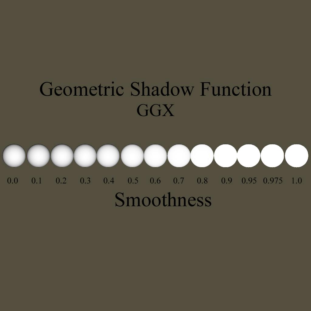
GGX GSF

This is a refactor of the Walter et al. GSF algorithm by multiplying the GSF by NdotV/NdotV.

float GGXGeometricShadowingFunction (float NdotL, float NdotV, float roughness){
    float roughnessSqr = roughness*roughness;
    float NdotLSqr = NdotL*NdotL;
    float NdotVSqr = NdotV*NdotV;


    float SmithL = (2 * NdotL)/ (NdotL + sqrt(roughnessSqr +
 ( 1-roughnessSqr) * NdotLSqr));
    float SmithV = (2 * NdotV)/ (NdotV + sqrt(roughnessSqr + 
( 1-roughnessSqr) * NdotVSqr));


	float Gs =  (SmithL * SmithV);
	return Gs;
}

GeometricShadow *= GGXGeometricShadowingFunction (NdotL, NdotV, roughness);

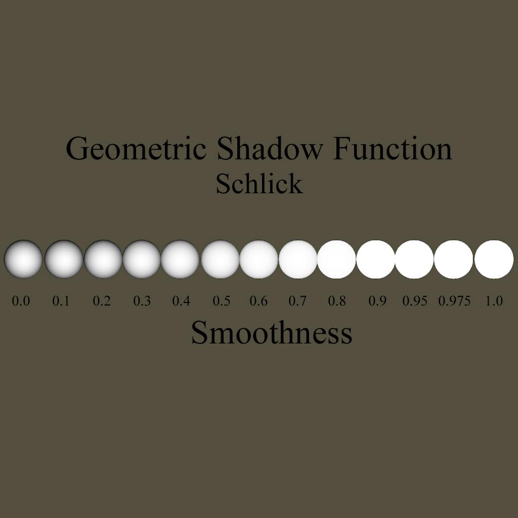
Schlick GSF

Schlick has made several approximations of the Smith GSF that can be applied to other Smith GSFs as well. This is the baseline Schlick Approximation of Smith GSF:

float SchlickGeometricShadowingFunction (float NdotL, float NdotV, float roughness)
{
    float roughnessSqr = roughness*roughness;


	float SmithL = (NdotL)/(NdotL * (1-roughnessSqr) + roughnessSqr);
	float SmithV = (NdotV)/(NdotV * (1-roughnessSqr) + roughnessSqr);


	return (SmithL * SmithV); 
}

GeometricShadow *= SchlickGeometricShadowingFunction (NdotL, NdotV, roughness);

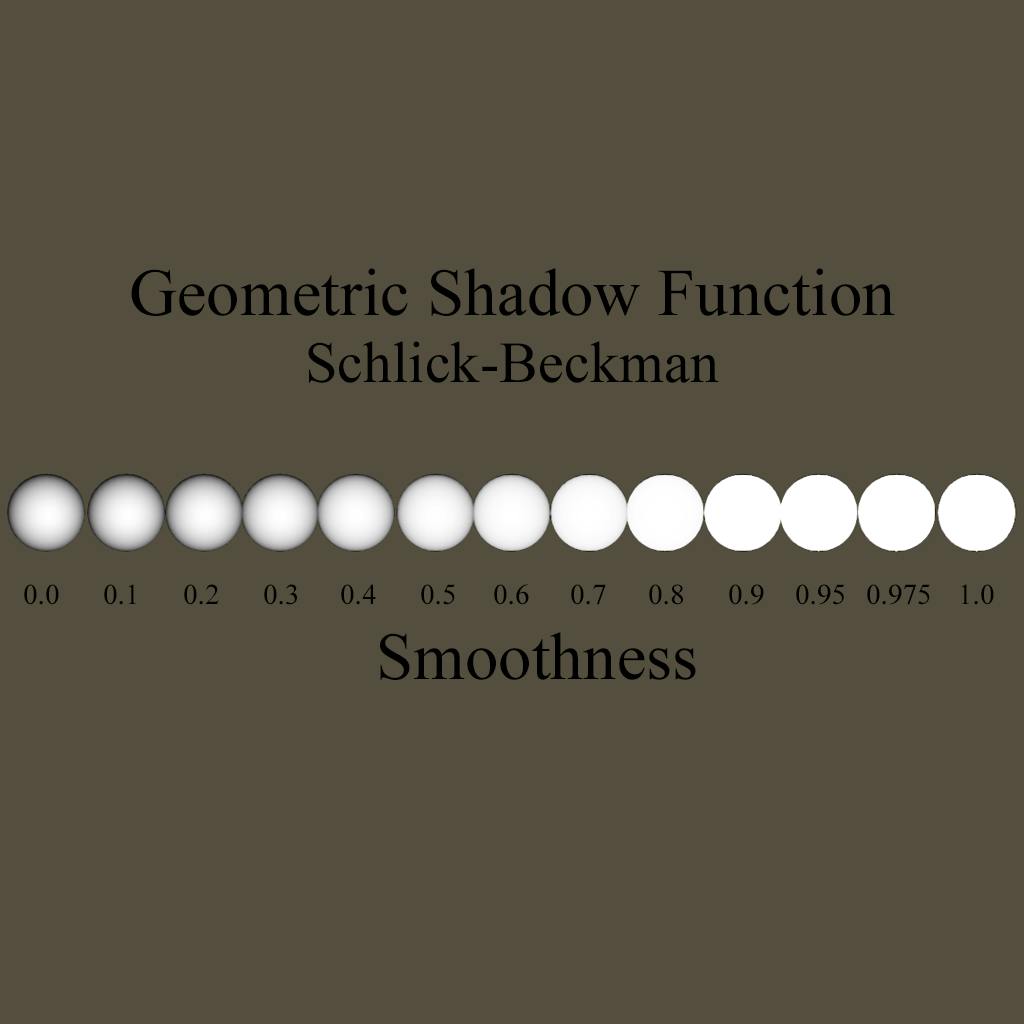
Schlick-Beckman GSF

This is the Schlick Approximation for the Beckman Function. It works by multiplying roughness by the square root of 2/PI, which instead of calcuating we just pre compute as 0.797884.....

float SchlickBeckmanGeometricShadowingFunction (float NdotL, float NdotV,
 float roughness){
    float roughnessSqr = roughness*roughness;
    float k = roughnessSqr * 0.797884560802865;


    float SmithL = (NdotL)/ (NdotL * (1- k) + k);
    float SmithV = (NdotV)/ (NdotV * (1- k) + k);


	float Gs =  (SmithL * SmithV);
	return Gs;
}

GeometricShadow *= SchlickBeckmanGeometricShadowingFunction (NdotL, NdotV, roughness);

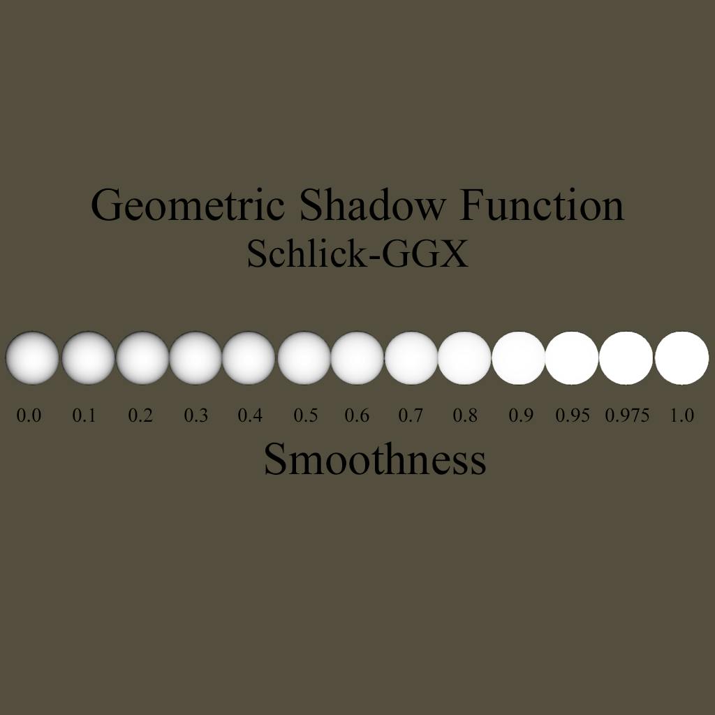
Schlick-GGX GSF

The Schlick Approximation of GGX simply divides our roughness value by two.

float SchlickGGXGeometricShadowingFunction (float NdotL, float NdotV, float roughness){
    float k = roughness / 2;


    float SmithL = (NdotL)/ (NdotL * (1- k) + k);
    float SmithV = (NdotV)/ (NdotV * (1- k) + k);


	float Gs =  (SmithL * SmithV);
	return Gs;
}

GeometricShadow *= SchlickGGXGeometricShadowingFunction (NdotL, NdotV, roughness);

Piecing Together Your PBR Shader Pt.3: The Fresnel Function

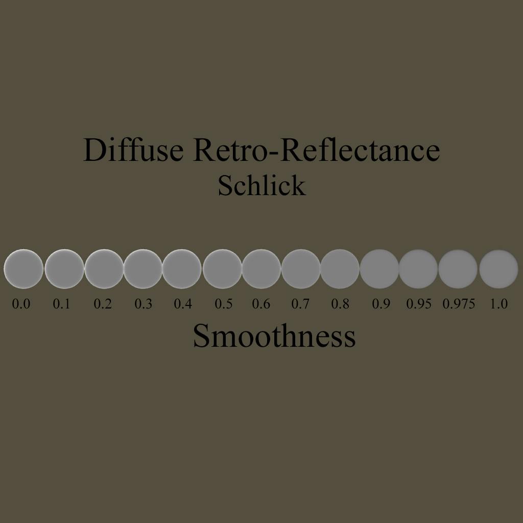
The Fresnel effect is named after the French physicist Augustin-Jean Fresnel who first described it. This effect states that the strength of reflections on a surface is dependent on the viewpoint. The amount of reflection increases on surfaces viewed at a grazing angle. In order to include the Fresnel effect into our shader we need to use it in several places. Firstly we need to account for the diffuse retro-reflection, and then we need to account for the BRDF Fresnel effect.

In order to calculate our Fresnel appropriately, we need to account for the normal incidence and grazing angles. We will use roughness below to calculate the diffuse Fresnel reflection incidence that we can pass into our Fresnel function. To calculate this we use a version of the Schlick approximation of Fresnel. The Schlick Approximation of Fresnel is constructed as:

schlick = x + (1-x) * pow(1-dotProduct,5);

This function can be approximated further into:

mix(x,1,pow(1-dotProduct,5));

This approximation may be faster on some GPUs. You can switch out the x and the 1 above to reverse the approximation, which we will do below to calculate our Diffuse.

float MixFunction(float i, float j, float x) {
	 return  j * x + i * (1.0 - x);
}

float SchlickFresnel(float i){
    float x = clamp(1.0-i, 0.0, 1.0);
    float x2 = x*x;
    return x2*x2*x;
}

//normal incidence reflection calculation
float F0 (float NdotL, float NdotV, float LdotH, float roughness){
    float FresnelLight = SchlickFresnel(NdotL); 
    float FresnelView = SchlickFresnel(NdotV);
    float FresnelDiffuse90 = 0.5 + 2.0 * LdotH*LdotH * roughness;
    return  MixFunction(1, FresnelDiffuse90, FresnelLight) * MixFunction(1, FresnelDiffuse90, FresnelView);
}

Schlick Fresnel

Schlick's Approximation of the Fresnel Equation may be one of his most famous approximations. This approximation of the Fresnel Effect allows us to calculate the reflectance at grazing angles.

float3 SchlickFresnelFunction(float3 SpecularColor,float LdotH){
    return SpecularColor + (1 - SpecularColor)* SchlickFresnel(LdotH);
}

FresnelFunction *=  SchlickFresnelFunction(specColor, LdotH);

This next algorithm relies on a specific value to be passed instead of the specular color. This new value is the Index of Refraction. The IOR is a dimensionless number used to describe the speed at which light passes through a surface. To enable this function we must add a new property and variable to our shader.

_Ior("Ior",  Range(1,4)) = 1.5

The above code belongs in the Shader Properties Section, while the line below should be placed with the other variables in the Public Variables Section.

float _Ior;

float SchlickIORFresnelFunction(float ior ,float LdotH){
    float f0 = pow(ior-1,2)/pow(ior+1, 2);
    return f0 + (1-f0) * SchlickFresnel(LdotH);
}

FresnelFunction *=  SchlickIORFresnelFunction(_Ior, LdotH);

Spherical-Gaussian Fresnel

The Spherical-Gaussian Fresnel function produces remarkably similar results to Schlicks Approximation. The only difference is that the power is derived from a Spherical Gaussian calculation.

float SphericalGaussianFresnelFunction(float LdotH,float SpecularColor)
{	
  float power = ((-5.55473 * LdotH) - 6.98316) * LdotH;
  return SpecularColor + (1 - SpecularColor) * pow(2,power);
}

FresnelFunction *= SphericalGaussianFresnelFunction(LdotH, specColor);

We've covered the primary algorithms that represent the different Geometric Shadowing Functions, as well as the pretty straightforward Fresnel Functions. In the next article we will be bringing all of these functions together to build our BRDF.